[R]2変量の散布図

# 2変量の散布図
png('test3.png')
plot(cars)
dev.off()

# 相関係数Rを求める
r = cor(cars$speed, cars$dist)
r

# 相関かどうかの検定
cor.test(cars$speed, cars$dist)

実行結果

$ Rscript test3.R
null device
  1
[1] 0.8068949

  Pearson's product-moment correlation

data: cars$speed and cars$dist
t = 9.464, df = 48, p-value = 1.49e-12
alternative hypothesis: true correlation is not equal to 0
95 percent confidence interval:
 0.6816422 0.8862036
sample estimates:
  cor
0.8068949

Pearson's product-moment correlationの内容

Parameter	Description
df	Degrees of Freedom
p-value	p値
95 percent confidence interval	95%信頼区間

出力結果

[R]単回帰分析

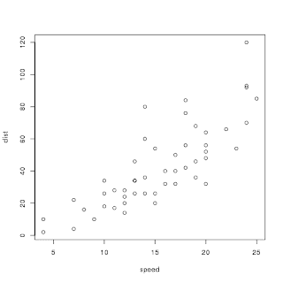
# 2変量の散布図
png('test1-0.png')
plot(cars)
dev.off()

# 単回帰分析（simple linear regression analysis）を行う
# lm: linear model
result <- lm(dist ~ speed, data=cars)
summary(result)

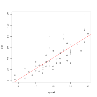
# 結果の直線を描画する
# abline(a, b): 切片a, 傾きb（y=a+bx）の直線を描く
# abline(result): resultにlm()の結果が入っている場合は回帰直線を描く
png('test1-1.png')
plot(cars)
abline(result, col="red")
dev.off()

実行結果

$ Rscript test1.R
null device
  1

Call:
lm(formula = dist ~ speed, data = cars)

Residuals:
  Min 1Q Median 3Q Max
-29.069 -9.525 -2.272 9.215 43.201

Coefficients:
  Estimate Std. Error t value Pr(>|t|)
(Intercept) -17.5791 6.7584 -2.601 0.0123 *
speed 3.9324 0.4155 9.464 1.49e-12 ***
---
Signif. codes: 0 ‘***’ 0.001 ‘**’ 0.01 ‘*’ 0.05 ‘.’ 0.1 ‘ ’ 1

Residual standard error: 15.38 on 48 degrees of freedom
Multiple R-squared: 0.6511, Adjusted R-squared: 0.6438
F-statistic: 89.57 on 1 and 48 DF, p-value: 1.49e-12

null device
  1

出力結果
test1-0.png

test1-1.png

[R]箱ひげ図

# 箱ひげ図を描く
x <- c(10, 20, 30, 40, 50, 30, 20)

png('test0.png')
boxplot(x)
dev.off()

出力結果